In early July, as the torrential rain that unleashed deadly flash flooding in the Texas Hill Country started to abate, a Kerr County resident standing on a bridge filmed something floating toward him through the trees. It was a cream-colored, ranch-style house with black trim — so perfectly intact it almost seemed like the swollen Guadalupe River might set it down and whoever owned it could pick up where they left off. “There’s a cat in there,” someone watching remarked.
Seconds later, the house plowed into the bridge, beams snapping as it crushed against the steel railing.
Kerr County appraisers estimate that thousands of homes like this one were damaged or destroyed by the July 4 floods, totaling more than $240 million in lost property value alone. In the end, the disaster killed more than 130 people and caused damage and economic losses worth $18 billion at minimum.
The tragedy in Texas is the latest addition to the country’s swelling disaster ledger, which is on track to well exceed $1 trillion this decade.
As countries continue to emit heat-trapping greenhouse gases, a warmer planet is fueling more severe hurricanes, wildfires, floods, droughts, and temperatures. Responding to — and rebuilding from — these disasters is costing Americans staggering amounts of money. The bigger the disaster, the wider the ripple of economic consequences.
Below are six graphs that demonstrate this growing disaster economy, from how much the federal government spends on relief to the rising prices of home insurance and building materials.
.fullwidth-video {
width: calc(100vw – 40px) !important;
position: relative !important;
left: 50% !important;
right: 50% !important;
margin-left: calc(-50vw + 20px) !important;
margin-right: calc(-50vw + 20px) !important;
max-width: none !important;
box-sizing: border-box !important;
}
.fullwidth-video video {
width: 100% !important;
height: auto !important;
max-width: none !important;
display: block !important;
border: 1px solid #3c3830 !important;
position: relative !important;
z-index: 2 !important;
}
.video__footer {
display: flex;
justify-content: flex-start;
align-items: flex-end;
margin-top: 8px;
margin-left: 0;
}
.video__credits {
display: flex;
flex-direction: column;
font-family: “Basis Grotesque”, sans-serif;
}
.video__source {
color: #777;
font-size: 12px;
margin-top: 0;
display: inline-block;
}
.video__credit {
color: #777;
font-size: 12px;
margin-top: 3px;
font-style: italic;
font-weight: bold;
display: inline-block;
}
document.addEventListener(‘DOMContentLoaded’, function() {
const video = document.getElementById(‘delayed-loop-video’);
video.addEventListener(‘ended’, function() {
setTimeout(() => {
video.currentTime = 0;
video.play();
}, 3000); // 3 second pause
});
});
Decades ago, two meteorologists at the National Oceanic and Atmospheric Administration started tracking the biggest natural disasters in the United States — the ones that incurred at least $1 billion in damages. The annual federal disaster counts have pointed in one direction since: up. Despite this worrying trend, the Trump administration this year directed NOAA to stop publishing data on billion-dollar disasters, destroying one of the clearest indicators of the growing cost of natural disasters on a warming planet.
.disaster-declarations {
–color-primary: #3c3830;
–color-secondary: #777;
–color-orange: #F79945;
–color-turquoise: #12A07F;
–color-fuchsia: #AC00E8;
–color-cobalt: #3977F3;
–color-earth: #3c3830;
–typography-primary: “PolySans”, Arial, sans-serif;
–typography-secondary: “Basis Grotesque”, Arial, sans-serif;
–spacing-base: 10px;
box-sizing: border-box;
font-family: var(–typography-secondary);
margin: 3rem auto 1.5rem auto;
padding: 0;
position: relative;
width: 100%;
}
.disaster-declarations * { box-sizing: border-box; }
.disaster-declarations__title {
font-family: var(–typography-primary);
font-size: 24px;
margin: var(–spacing-base) 0;
}
.disaster-declarations__subtitle {
font-family: var(–typography-secondary);
color: var(–color-primary);
font-size: 18px;
margin: 0 0 var(–spacing-base);
}
.disaster-declarations__axis-label {
color: var(–color-primary);
font-size: 14px;
}
.axis-grid line {
stroke: #e0e0e0;
stroke-opacity: 0.7;
shape-rendering: crispEdges;
}
.axis-grid .domain { stroke: none; }
.line { fill: none; stroke-width: 2.5px; }
.pulsing-dot { stroke: white; stroke-width: 1.7px; }
.data-label {
font-family: var(–typography-secondary);
font-size: 11px;
fill: var(–color-primary);
}
.disaster-declarations__footer { display: flex; justify-content: space-between; align-items: flex-end; margin-top: 8px; }
.disaster-declarations__credits { display: flex; flex-direction: column; }
.disaster-declarations__source { color: var(–color-secondary); font-size: 12px; margin-top: 0; display: inline-block; }
.disaster-declarations__credit { color: var(–color-secondary); font-size: 12px; margin-top: 3px; font-style: italic; font-weight: bold; display: inline-block; }
.disaster-declarations__logo { height: 20px; width: auto; margin-left: auto; padding-right: 20px; margin-right: 0; margin-bottom: 0; }
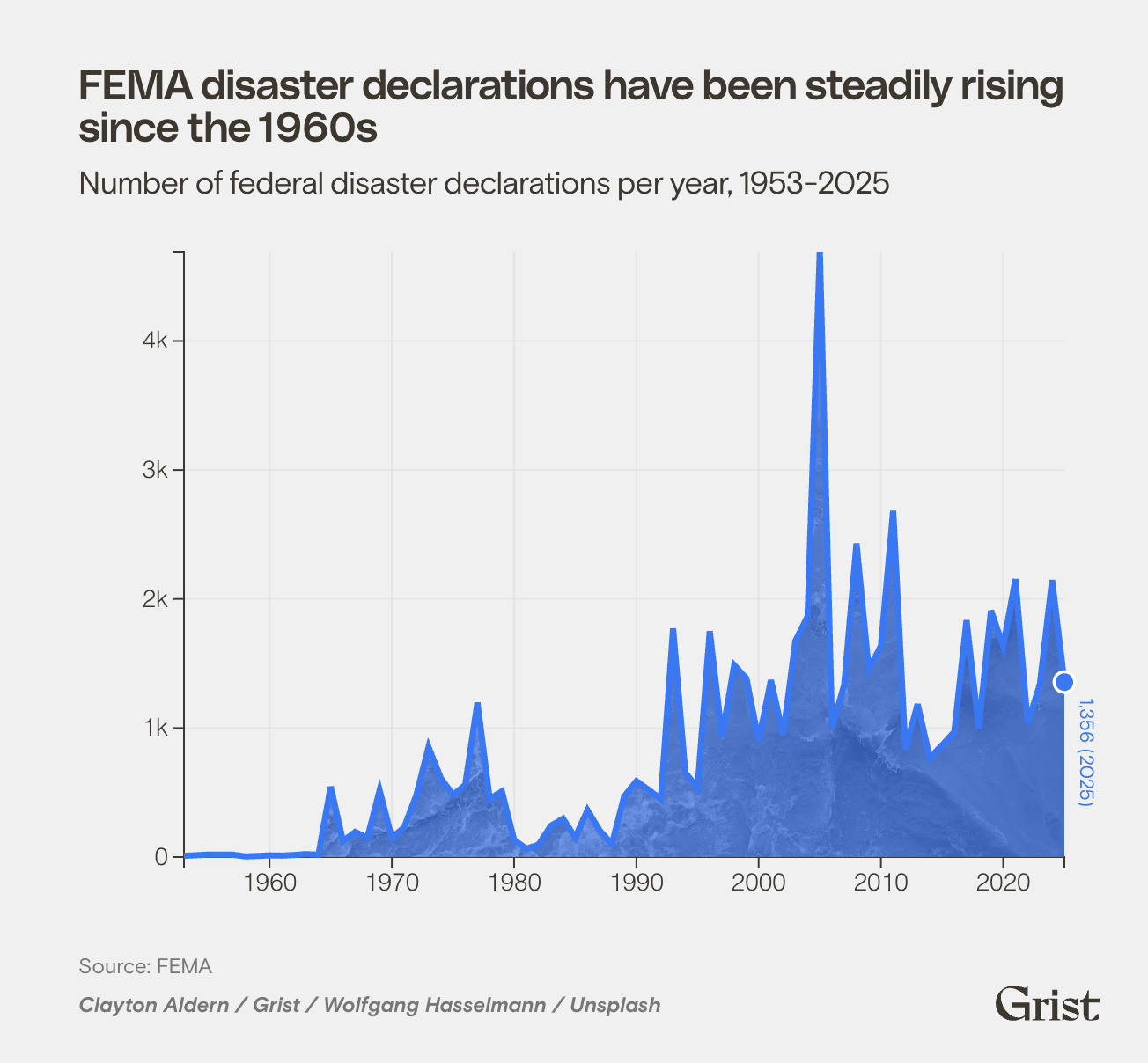
FEMA disaster declarations have been steadily rising since the 1960s
Number of federal disaster declarations per year, 1953-2025
(function() {
const INIT_KEY = ‘__grist_disaster_declarations_initialized__’;
if (window[INIT_KEY]) { return; }
window[INIT_KEY] = true;
const DECLARATION_COLORS = {
TEXT: ‘var(–color-primary)’,
LINE: ‘#3977F3’
};
const initialSvgHeight = 400;
const svg = d3.select(‘#declarations-chart’);
const formatCompactWithB = (n) => d3.format(‘~s’)(n).replace(‘G’, ‘B’);
const rawData = [
{ year: 1953, count: 10 },
{ year: 1954, count: 14 },
{ year: 1955, count: 19 },
{ year: 1956, count: 18 },
{ year: 1957, count: 18 },
{ year: 1958, count: 5 },
{ year: 1959, count: 8 },
{ year: 1960, count: 13 },
{ year: 1961, count: 11 },
{ year: 1962, count: 16 },
{ year: 1963, count: 23 },
{ year: 1964, count: 18 },
{ year: 1965, count: 545 },
{ year: 1966, count: 124 },
{ year: 1967, count: 194 },
{ year: 1968, count: 149 },
{ year: 1969, count: 516 },
{ year: 1970, count: 149 },
{ year: 1971, count: 230 },
{ year: 1972, count: 478 },
{ year: 1973, count: 852 },
{ year: 1974, count: 612 },
{ year: 1975, count: 482 },
{ year: 1976, count: 558 },
{ year: 1977, count: 1197 },
{ year: 1978, count: 451 },
{ year: 1979, count: 509 },
{ year: 1980, count: 132 },
{ year: 1981, count: 65 },
{ year: 1982, count: 97 },
{ year: 1983, count: 242 },
{ year: 1984, count: 297 },
{ year: 1985, count: 152 },
{ year: 1986, count: 363 },
{ year: 1987, count: 206 },
{ year: 1988, count: 100 },
{ year: 1989, count: 470 },
{ year: 1990, count: 588 },
{ year: 1991, count: 521 },
{ year: 1992, count: 449 },
{ year: 1993, count: 1772 },
{ year: 1994, count: 656 },
{ year: 1995, count: 533 },
{ year: 1996, count: 1750 },
{ year: 1997, count: 936 },
{ year: 1998, count: 1487 },
{ year: 1999, count: 1384 },
{ year: 2000, count: 901 },
{ year: 2001, count: 1371 },
{ year: 2002, count: 945 },
{ year: 2003, count: 1673 },
{ year: 2004, count: 1863 },
{ year: 2005, count: 4692 },
{ year: 2006, count: 1002 },
{ year: 2007, count: 1337 },
{ year: 2008, count: 2430 },
{ year: 2009, count: 1456 },
{ year: 2010, count: 1637 },
{ year: 2011, count: 2684 },
{ year: 2012, count: 835 },
{ year: 2013, count: 1185 },
{ year: 2014, count: 766 },
{ year: 2015, count: 868 },
{ year: 2016, count: 968 },
{ year: 2017, count: 1835 },
{ year: 2018, count: 997 },
{ year: 2019, count: 1910 },
{ year: 2020, count: 1635 },
{ year: 2021, count: 2154 },
{ year: 2022, count: 1037 },
{ year: 2023, count: 1338 },
{ year: 2024, count: 2147 },
{ year: 2025, count: 1356 }
];
const data = rawData.map(d => ({ year: new Date(+d.year, 0, 1), count: +d.count }));
const margin = { top: 20, right: 40, bottom: 36, left: window.innerWidth x(d.year))
.y(d => y(d.count));
x.domain(d3.extent(data, d => d.year));
y.domain([0, d3.max(data, d => d.count)]);
svg.attr(‘height’, initialSvgHeight);
// Compute a dynamic year interval for ticks to avoid label collisions
const startYear = data[0].year.getFullYear();
const endYear = data[data.length – 1].year.getFullYear();
const totalYears = endYear – startYear;
const minLabelSpacingPx = 60;
const maxTicks = Math.max(2, Math.floor(width / minLabelSpacingPx));
const approxYearsPerTick = Math.max(1, Math.ceil(totalYears / maxTicks));
const niceSteps = [1, 2, 5, 10, 20, 25, 50, 100];
const stepYears = niceSteps.find(s => s >= approxYearsPerTick) || niceSteps[niceSteps.length – 1];
const xTickInterval = d3.timeYear.every(stepYears);
// Gridlines
svg.append(‘g’)
.attr(‘class’, ‘axis-grid’)
.attr(‘transform’, `translate(${margin.left},${height + margin.top})`)
.call(d3.axisBottom(x).ticks(xTickInterval).tickSize(-height).tickFormat(”));
svg.append(‘g’)
.attr(‘class’, ‘axis-grid’)
.attr(‘transform’, `translate(${margin.left},${margin.top})`)
.call(d3.axisLeft(y).ticks(5).tickSize(-width).tickFormat(”));
const xAxis = g => g
.attr(‘transform’, `translate(${margin.left},${height + margin.top})`)
.call(d3.axisBottom(x).ticks(xTickInterval).tickFormat(d3.timeFormat(‘%Y’)))
.selectAll(‘text’)
.attr(‘class’, ‘disaster-declarations__axis-label’)
.style(‘fill’, DECLARATION_COLORS.TEXT)
.style(‘text-anchor’, ‘middle’);
const yAxis = g => g
.attr(‘transform’, `translate(${margin.left},${margin.top})`)
.call(d3.axisLeft(y).ticks(5).tickFormat(d => d3.format(‘~s’)(d)))
.selectAll(‘text’)
.attr(‘class’, ‘disaster-declarations__axis-label’)
.style(‘fill’, DECLARATION_COLORS.TEXT);
svg.append(‘g’).call(xAxis);
svg.append(‘g’).call(yAxis);
const chart = svg.append(‘g’).attr(‘transform’, `translate(${margin.left},${margin.top})`);
// Image area fill under the line
const area = d3.area()
.x(d => x(d.year))
.y0(y(0))
.y1(d => y(d.count));
const defs = chart.append(‘defs’);
const grayFilter = defs.append(‘filter’).attr(‘id’, ‘declarationsGreyscale’);
grayFilter.append(‘feColorMatrix’).attr(‘type’, ‘saturate’).attr(‘values’, ‘0’);
const areaMask = defs.append(‘mask’).attr(‘id’, ‘declarationsAreaMask’);
areaMask.append(‘path’)
.attr(‘d’, area(data))
.attr(‘fill’, ‘white’);
chart.append(‘image’)
.attr(‘xlink:href’, ‘https://grist.org/wp-content/uploads/2025/08/wolfgang-hasselmann-sqJ5mnQ7wmM-unsplash.jpg’)
.attr(‘x’, 0)
.attr(‘y’, 0)
.attr(‘width’, width)
.attr(‘height’, height)
.attr(‘preserveAspectRatio’, ‘xMidYMid slice’)
.attr(‘mask’, ‘url(#declarationsAreaMask)’)
.attr(‘filter’, ‘url(#declarationsGreyscale)’);
// Color overlay for the area
chart.append(‘path’)
.datum(data)
.attr(‘d’, area)
.attr(‘fill’, DECLARATION_COLORS.LINE)
.style(‘opacity’, 0.65);
// Main line
chart.append(‘path’)
.datum(data)
.attr(‘class’, ‘line’)
.attr(‘d’, line)
.style(‘stroke’, DECLARATION_COLORS.LINE);
const last = data[data.length – 1];
const dotRadius = 5;
const circle = chart.append(‘circle’)
.attr(‘class’, ‘pulsing-dot’)
.attr(‘cx’, x(last.year))
.attr(‘cy’, y(last.count))
.attr(‘r’, dotRadius)
.style(‘fill’, DECLARATION_COLORS.LINE);
function animatePulse() {
circle.transition().duration(750).attr(‘r’, dotRadius * 1.2)
.transition().duration(750).attr(‘r’, dotRadius).on(‘end’, animatePulse);
}
animatePulse();
const label = chart.append(‘text’)
.attr(‘class’, ‘data-label’)
.attr(‘x’, x(last.year) + dotRadius + 4)
.attr(‘y’, y(last.count) + dotRadius + 4)
.attr(‘text-anchor’, ‘start’)
.attr(‘transform’, `rotate(90, ${x(last.year) + dotRadius + 4}, ${y(last.count) + dotRadius + 4})`)
.style(‘fill’, DECLARATION_COLORS.LINE)
.text(`${d3.format(‘,’)(last.count)} (${last.year.getFullYear()})`);
}
if (document.readyState === ‘loading’) {
document.addEventListener(‘DOMContentLoaded’, renderChart);
} else {
renderChart();
}
window.addEventListener(‘resize’, renderChart);
})();
In its first decade of existence, FEMA handled 25 major disaster declarations per year on average. In the past decade, as disasters have carved larger paths through denser communities and more expensive infrastructure, the agency has had to field 63 declarations annually — a 150 percent increase.
.fema-spending {
–color-primary: #3c3830;
–color-secondary: #777;
–color-orange: #F79945;
–color-turquoise: #12A07F;
–color-fuchsia: #AC00E8;
–color-cobalt: #3977F3;
–color-earth: #3c3830;
–typography-primary: “PolySans”, Arial, sans-serif;
–typography-secondary: “Basis Grotesque”, Arial, sans-serif;
–spacing-base: 10px;
box-sizing: border-box;
font-family: var(–typography-secondary);
margin: 3rem auto 1.5rem auto;
padding: 0;
position: relative;
width: 100%;
}
.fema-spending * { box-sizing: border-box; }
.fema-spending__title {
font-family: var(–typography-primary);
font-size: 24px;
margin: var(–spacing-base) 0;
}
.fema-spending__subtitle {
font-family: var(–typography-secondary);
color: var(–color-primary);
font-size: 18px;
margin: 0 0 var(–spacing-base);
}
.fema-spending__axis-label {
color: var(–color-primary);
font-size: 14px;
}
.axis-grid line {
stroke: #e0e0e0;
stroke-opacity: 0.7;
shape-rendering: crispEdges;
}
.axis-grid .domain { stroke: none; }
.line { fill: none; stroke-width: 2.5px; }
.pulsing-dot { stroke: white; stroke-width: 1.7px; }
.data-label {
font-family: var(–typography-secondary);
font-size: 11px;
fill: var(–color-primary);
}
.fema-spending__footer { display: flex; justify-content: space-between; align-items: flex-end; margin-top: 8px; }
.fema-spending__credits { display: flex; flex-direction: column; }
.fema-spending__source { color: var(–color-secondary); font-size: 12px; margin-top: 0; display: inline-block; }
.fema-spending__credit { color: var(–color-secondary); font-size: 12px; margin-top: 3px; font-style: italic; font-weight: bold; display: inline-block; }
.fema-spending__logo { height: 20px; width: auto; margin-left: auto; padding-right: 20px; margin-right: 0; margin-bottom: 0; }
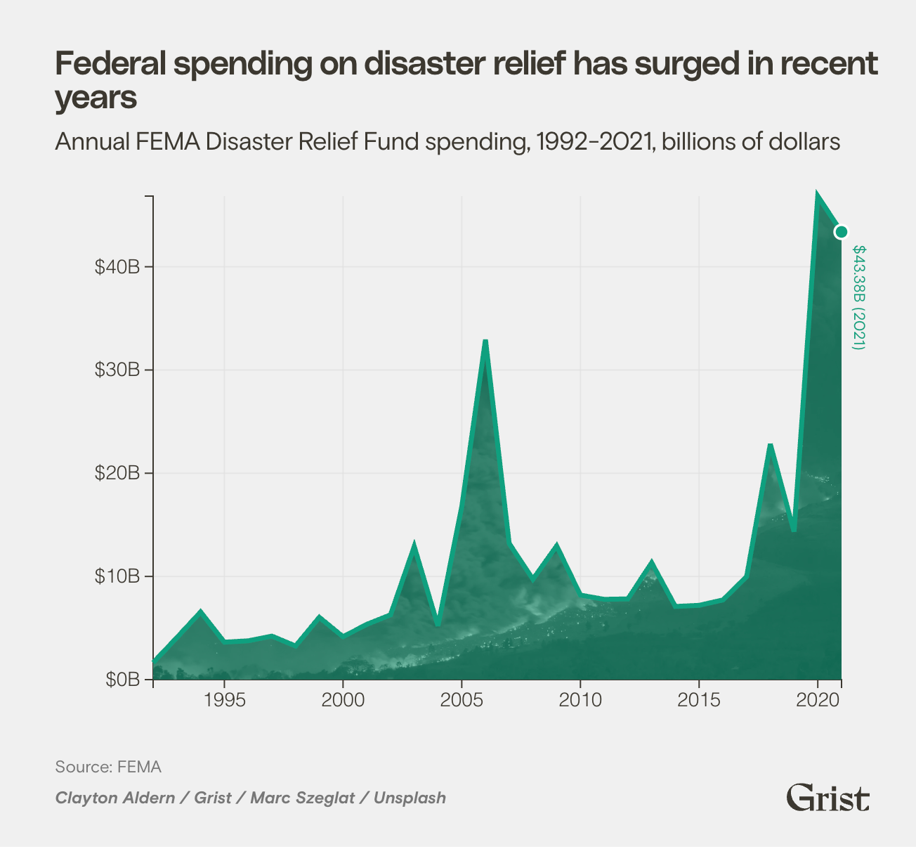
Federal spending on disaster relief has surged in recent years
Annual FEMA Disaster Relief Fund spending, 1992-2021, billions of dollars
(function() {
const INIT_KEY = ‘__grist_fema_spending_initialized__’;
if (window[INIT_KEY]) { return; }
window[INIT_KEY] = true;
const COLORS = {
TEXT: ‘var(–color-primary)’,
LINE: ‘var(–color-turquoise)’
};
const initialSvgHeight = 400;
const svg = d3.select(‘#spending-chart’);
const rawData = [
{ year: 1992, spent: 1.65 },
{ year: 1993, spent: 4.08 },
{ year: 1994, spent: 6.56 },
{ year: 1995, spent: 3.63 },
{ year: 1996, spent: 3.76 },
{ year: 1997, spent: 4.22 },
{ year: 1998, spent: 3.26 },
{ year: 1999, spent: 6.04 },
{ year: 2000, spent: 4.16 },
{ year: 2001, spent: 5.36 },
{ year: 2002, spent: 6.28 },
{ year: 2003, spent: 12.90 },
{ year: 2004, spent: 5.21 },
{ year: 2005, spent: 16.75 },
{ year: 2006, spent: 32.94 },
{ year: 2007, spent: 13.20 },
{ year: 2008, spent: 9.73 },
{ year: 2009, spent: 12.96 },
{ year: 2010, spent: 8.19 },
{ year: 2011, spent: 7.78 },
{ year: 2012, spent: 7.82 },
{ year: 2013, spent: 11.33 },
{ year: 2014, spent: 7.09 },
{ year: 2015, spent: 7.20 },
{ year: 2016, spent: 7.72 },
{ year: 2017, spent: 9.97 },
{ year: 2018, spent: 22.83 },
{ year: 2019, spent: 14.34 },
{ year: 2020, spent: 46.85 },
{ year: 2021, spent: 43.38 }
];
const data = rawData.map(d => ({ year: new Date(+d.year, 0, 1), spent: +d.spent }));
const margin = { top: 20, right: 40, bottom: 36, left: window.innerWidth x(d.year))
.y(d => y(d.spent));
x.domain(d3.extent(data, d => d.year));
y.domain([0, d3.max(data, d => d.spent)]);
svg.attr(‘height’, initialSvgHeight);
// Compute a dynamic year interval for ticks
const startYear = data[0].year.getFullYear();
const endYear = data[data.length – 1].year.getFullYear();
const totalYears = endYear – startYear;
const minLabelSpacingPx = 60;
const maxTicks = Math.max(2, Math.floor(width / minLabelSpacingPx));
const approxYearsPerTick = Math.max(1, Math.ceil(totalYears / maxTicks));
const niceSteps = [1, 2, 5, 10, 20, 25, 50, 100];
const stepYears = niceSteps.find(s => s >= approxYearsPerTick) || niceSteps[niceSteps.length – 1];
const xTickInterval = d3.timeYear.every(stepYears);
// Gridlines
svg.append(‘g’)
.attr(‘class’, ‘axis-grid’)
.attr(‘transform’, `translate(${margin.left},${height + margin.top})`)
.call(d3.axisBottom(x).ticks(xTickInterval).tickSize(-height).tickFormat(”));
svg.append(‘g’)
.attr(‘class’, ‘axis-grid’)
.attr(‘transform’, `translate(${margin.left},${margin.top})`)
.call(d3.axisLeft(y).ticks(5).tickSize(-width).tickFormat(”));
const xAxis = g => g
.attr(‘transform’, `translate(${margin.left},${height + margin.top})`)
.call(d3.axisBottom(x).ticks(xTickInterval).tickFormat(d3.timeFormat(‘%Y’)))
.selectAll(‘text’)
.attr(‘class’, ‘fema-spending__axis-label’)
.style(‘fill’, COLORS.TEXT)
.style(‘text-anchor’, ‘middle’);
const yAxis = g => g
.attr(‘transform’, `translate(${margin.left},${margin.top})`)
.call(d3.axisLeft(y).ticks(5).tickFormat(d => `$${d}B`))
.selectAll(‘text’)
.attr(‘class’, ‘fema-spending__axis-label’)
.style(‘fill’, COLORS.TEXT);
svg.append(‘g’).call(xAxis);
svg.append(‘g’).call(yAxis);
const chart = svg.append(‘g’).attr(‘transform’, `translate(${margin.left},${margin.top})`);
// Image area fill under the line
const area = d3.area()
.x(d => x(d.year))
.y0(y(0))
.y1(d => y(d.spent));
const defs = chart.append(‘defs’);
const grayFilter = defs.append(‘filter’).attr(‘id’, ‘spendingGreyscale’);
grayFilter.append(‘feColorMatrix’).attr(‘type’, ‘saturate’).attr(‘values’, ‘0’);
const areaMask = defs.append(‘mask’).attr(‘id’, ‘spendingAreaMask’);
areaMask.append(‘path’)
.attr(‘d’, area(data))
.attr(‘fill’, ‘white’);
chart.append(‘image’)
.attr(‘xlink:href’, ‘https://grist.org/wp-content/uploads/2025/08/marc-szeglat-BsAzhHIIwxg-unsplash.jpg’)
.attr(‘x’, 0)
.attr(‘y’, 0)
.attr(‘width’, width)
.attr(‘height’, height)
.attr(‘preserveAspectRatio’, ‘xMidYMid slice’)
.attr(‘mask’, ‘url(#spendingAreaMask)’)
.attr(‘filter’, ‘url(#spendingGreyscale)’);
// Color overlay for the area
chart.append(‘path’)
.datum(data)
.attr(‘d’, area)
.attr(‘fill’, COLORS.LINE)
.style(‘opacity’, 0.65);
// Main line
chart.append(‘path’)
.datum(data)
.attr(‘class’, ‘line’)
.attr(‘d’, line)
.style(‘stroke’, COLORS.LINE);
const last = data[data.length – 1];
const dotRadius = 5;
const circle = chart.append(‘circle’)
.attr(‘class’, ‘pulsing-dot’)
.attr(‘cx’, x(last.year))
.attr(‘cy’, y(last.spent))
.attr(‘r’, dotRadius)
.style(‘fill’, COLORS.LINE);
function animatePulse() {
circle.transition().duration(750).attr(‘r’, dotRadius * 1.2)
.transition().duration(750).attr(‘r’, dotRadius).on(‘end’, animatePulse);
}
animatePulse();
const label = chart.append(‘text’)
.attr(‘class’, ‘data-label’)
.attr(‘x’, x(last.year) + dotRadius + 4)
.attr(‘y’, y(last.spent) + dotRadius + 4)
.attr(‘text-anchor’, ‘start’)
.attr(‘transform’, `rotate(90, ${x(last.year) + dotRadius + 4}, ${y(last.spent) + dotRadius + 4})`)
.style(‘fill’, COLORS.LINE)
.text(`$${last.spent}B (${last.year.getFullYear()})`);
}
if (document.readyState === ‘loading’) {
document.addEventListener(‘DOMContentLoaded’, renderChart);
} else {
renderChart();
}
window.addEventListener(‘resize’, renderChart);
})();
Federal Emergency Management Agency spending on disasters, including the COVID-19 public health crisis, has averaged $12 billion over the past 30 years. But the average obscures a concerning trend underway: The number of very large disasters is rising, corresponding with a significant uptick in the share spent specifically on response and recovery. Between 1992 and 2004, the agency’s Disaster Relief Fund, a federally appropriated pot of money for disaster response operations, averaged $3.4 billion per year. Now, annual spending is closer to $16 billion, as disasters get more intense and the number of people and amount of infrastructure in at-risk areas rises.
.construction-index {
–color-primary: #3c3830;
–color-secondary: #777;
–color-orange: #F79945;
–color-turquoise: #12A07F;
–color-fuchsia: #AC00E8;
–color-cobalt: #3977F3;
–color-earth: #3c3830;
–typography-primary: “PolySans”, Arial, sans-serif;
–typography-secondary: “Basis Grotesque”, Arial, sans-serif;
–spacing-base: 10px;
box-sizing: border-box;
font-family: var(–typography-secondary);
margin: 3rem auto 1.5rem auto;
padding: 0;
position: relative;
width: 100%;
}
.construction-index * { box-sizing: border-box; }
.construction-index__title {
font-family: var(–typography-primary);
font-size: 24px;
margin: var(–spacing-base) 0;
}
.construction-index__subtitle {
font-family: var(–typography-secondary);
color: var(–color-primary);
font-size: 18px;
margin: 0 0 var(–spacing-base);
}
.construction-index__axis-label {
color: var(–color-primary);
font-size: 14px;
}
.axis-grid line {
stroke: #e0e0e0;
stroke-opacity: 0.7;
shape-rendering: crispEdges;
}
.axis-grid .domain { stroke: none; }
.line { fill: none; stroke-width: 2.5px; }
.pulsing-dot { stroke: white; stroke-width: 1.7px; }
.data-label {
font-family: var(–typography-secondary);
font-size: 11px;
fill: var(–color-primary);
}
.construction-index__footer { display: flex; justify-content: space-between; align-items: flex-end; margin-top: 8px; }
.construction-index__credits { display: flex; flex-direction: column; }
.construction-index__source { color: var(–color-secondary); font-size: 12px; margin-top: 0; display: inline-block; }
.construction-index__credit { color: var(–color-secondary); font-size: 12px; margin-top: 3px; font-style: italic; font-weight: bold; display: inline-block; }
.construction-index__logo { height: 20px; width: auto; margin-left: auto; padding-right: 20px; margin-right: 0; margin-bottom: 0; }
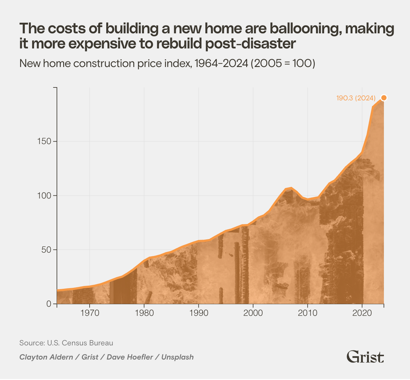
The costs of building a new home are ballooning, making it more expensive to rebuild post-disaster
New home construction price index, 1964-2024 (2005 = 100)
(function() {
const INIT_KEY = ‘__grist_construction_index_initialized__’;
if (window[INIT_KEY]) { return; }
window[INIT_KEY] = true;
const COLORS = {
TEXT: ‘var(–color-primary)’,
LINE: ‘var(–color-orange)’
};
const initialSvgHeight = 400;
const svg = d3.select(‘#construction-chart’);
const rawData = [
{ year: 1964, index: 12.4 },
{ year: 1965, index: 12.8 },
{ year: 1966, index: 13.4 },
{ year: 1967, index: 13.8 },
{ year: 1968, index: 14.6 },
{ year: 1969, index: 15.5 },
{ year: 1970, index: 15.9 },
{ year: 1971, index: 16.8 },
{ year: 1972, index: 18 },
{ year: 1973, index: 19.8 },
{ year: 1974, index: 21.8 },
{ year: 1975, index: 23.7 },
{ year: 1976, index: 25.2 },
{ year: 1977, index: 28.2 },
{ year: 1978, index: 31.7 },
{ year: 1979, index: 35.7 },
{ year: 1980, index: 39.8 },
{ year: 1981, index: 42.6 },
{ year: 1982, index: 43.4 },
{ year: 1983, index: 44.7 },
{ year: 1984, index: 46.7 },
{ year: 1985, index: 47.9 },
{ year: 1986, index: 50.4 },
{ year: 1987, index: 52.7 },
{ year: 1988, index: 54.5 },
{ year: 1989, index: 56.4 },
{ year: 1990, index: 58 },
{ year: 1991, index: 58.2 },
{ year: 1992, index: 58.9 },
{ year: 1993, index: 61.8 },
{ year: 1994, index: 64.6 },
{ year: 1995, index: 67.3 },
{ year: 1996, index: 68.6 },
{ year: 1997, index: 70.6 },
{ year: 1998, index: 72.5 },
{ year: 1999, index: 72.7 },
{ year: 2000, index: 75.9 },
{ year: 2001, index: 79.7 },
{ year: 2002, index: 81.7 },
{ year: 2003, index: 85.9 },
{ year: 2004, index: 93.1 },
{ year: 2005, index: 100 },
{ year: 2006, index: 106 },
{ year: 2007, index: 107 },
{ year: 2008, index: 103.3 },
{ year: 2009, index: 98.1 },
{ year: 2010, index: 96.4 },
{ year: 2011, index: 97.4 },
{ year: 2012, index: 98.4 },
{ year: 2013, index: 104.8 },
{ year: 2014, index: 111.2 },
{ year: 2015, index: 114 },
{ year: 2016, index: 119.8 },
{ year: 2017, index: 125.9 },
{ year: 2018, index: 130.4 },
{ year: 2019, index: 134.4 },
{ year: 2020, index: 139.8 },
{ year: 2021, index: 156 },
{ year: 2022, index: 181.8 },
{ year: 2023, index: 186.3 },
{ year: 2024, index: 190.3 }
];
const data = rawData.map(d => ({ year: new Date(+d.year, 0, 1), index: +d.index }));
const margin = { top: 20, right: 20, bottom: 36, left: window.innerWidth x(d.year))
.y(d => y(d.index));
x.domain(d3.extent(data, d => d.year));
y.domain([0, d3.max(data, d => d.index) * 1.05]);
svg.attr(‘height’, initialSvgHeight);
// Compute a dynamic year interval for ticks
const startYear = data[0].year.getFullYear();
const endYear = data[data.length – 1].year.getFullYear();
const totalYears = endYear – startYear;
const minLabelSpacingPx = 60;
const maxTicks = Math.max(2, Math.floor(width / minLabelSpacingPx));
const approxYearsPerTick = Math.max(1, Math.ceil(totalYears / maxTicks));
const niceSteps = [1, 2, 5, 10, 20, 25, 50, 100];
const stepYears = niceSteps.find(s => s >= approxYearsPerTick) || niceSteps[niceSteps.length – 1];
const xTickInterval = d3.timeYear.every(stepYears);
// Gridlines
svg.append(‘g’)
.attr(‘class’, ‘axis-grid’)
.attr(‘transform’, `translate(${margin.left},${height + margin.top})`)
.call(d3.axisBottom(x).ticks(xTickInterval).tickSize(-height).tickFormat(”));
svg.append(‘g’)
.attr(‘class’, ‘axis-grid’)
.attr(‘transform’, `translate(${margin.left},${margin.top})`)
.call(d3.axisLeft(y).ticks(5).tickSize(-width).tickFormat(”));
const xAxis = g => g
.attr(‘transform’, `translate(${margin.left},${height + margin.top})`)
.call(d3.axisBottom(x).ticks(xTickInterval).tickFormat(d3.timeFormat(‘%Y’)))
.selectAll(‘text’)
.attr(‘class’, ‘construction-index__axis-label’)
.style(‘fill’, COLORS.TEXT)
.style(‘text-anchor’, ‘middle’);
const yAxis = g => g
.attr(‘transform’, `translate(${margin.left},${margin.top})`)
.call(d3.axisLeft(y).ticks(5).tickFormat(d => d))
.selectAll(‘text’)
.attr(‘class’, ‘construction-index__axis-label’)
.style(‘fill’, COLORS.TEXT);
svg.append(‘g’).call(xAxis);
svg.append(‘g’).call(yAxis);
const chart = svg.append(‘g’).attr(‘transform’, `translate(${margin.left},${margin.top})`);
// Image area fill under the line
const area = d3.area()
.x(d => x(d.year))
.y0(y(0))
.y1(d => y(d.index));
const defs = chart.append(‘defs’);
const grayFilter = defs.append(‘filter’).attr(‘id’, ‘constructionGreyscale’);
grayFilter.append(‘feColorMatrix’).attr(‘type’, ‘saturate’).attr(‘values’, ‘0’);
const areaMask = defs.append(‘mask’).attr(‘id’, ‘constructionAreaMask’);
areaMask.append(‘path’)
.attr(‘d’, area(data))
.attr(‘fill’, ‘white’);
chart.append(‘image’)
.attr(‘xlink:href’, ‘https://grist.org/wp-content/uploads/2025/08/dave-hoefler-MrxlMcZxqhY-unsplash.jpg’)
.attr(‘x’, 0)
.attr(‘y’, 0)
.attr(‘width’, width)
.attr(‘height’, height)
.attr(‘preserveAspectRatio’, ‘xMidYMid slice’)
.attr(‘mask’, ‘url(#constructionAreaMask)’)
.attr(‘filter’, ‘url(#constructionGreyscale)’);
// Color overlay for the area
chart.append(‘path’)
.datum(data)
.attr(‘d’, area)
.attr(‘fill’, COLORS.LINE)
.style(‘opacity’, 0.65);
// Main line
chart.append(‘path’)
.datum(data)
.attr(‘class’, ‘line’)
.attr(‘d’, line)
.style(‘stroke’, COLORS.LINE);
const last = data[data.length – 1];
const dotRadius = 5;
const circle = chart.append(‘circle’)
.attr(‘class’, ‘pulsing-dot’)
.attr(‘cx’, x(last.year))
.attr(‘cy’, y(last.index))
.attr(‘r’, dotRadius)
.style(‘fill’, COLORS.LINE);
function animatePulse() {
circle.transition().duration(750).attr(‘r’, dotRadius * 1.2)
.transition().duration(750).attr(‘r’, dotRadius).on(‘end’, animatePulse);
}
animatePulse();
const label = chart.append(‘text’)
.attr(‘class’, ‘data-label’)
.attr(‘y’, y(last.index) + 4)
.style(‘fill’, COLORS.LINE)
.text(`${last.index} (${last.year.getFullYear()})`);
const rightX = x(last.year) + 8 + dotRadius;
const labelWidth = label.node().getComputedTextLength();
if (rightX + labelWidth > width) {
label
.attr(‘text-anchor’, ‘end’)
.attr(‘x’, x(last.year) – 8 – dotRadius);
} else {
label
.attr(‘text-anchor’, ‘start’)
.attr(‘x’, rightX);
}
}
if (document.readyState === ‘loading’) {
document.addEventListener(‘DOMContentLoaded’, renderChart);
} else {
renderChart();
}
window.addEventListener(‘resize’, renderChart);
})();
Disasters often require homeowners to rebuild from the ground up, but the cost of constructing a new home has nearly doubled since 1996 (after adjusting for inflation). So as extreme weather becomes more intense, rising building costs are making it even more difficult for families to recover.
.insurance-premiums {
–color-primary: #3c3830;
–color-secondary: #777;
–color-orange: #F79945;
–color-turquoise: #12A07F;
–color-fuchsia: #AC00E8;
–color-cobalt: #3977F3;
–color-earth: #3c3830;
–typography-primary: “PolySans”, Arial, sans-serif;
–typography-secondary: “Basis Grotesque”, Arial, sans-serif;
–spacing-base: 10px;
box-sizing: border-box;
font-family: var(–typography-secondary);
margin: 3rem auto 1.5rem auto;
padding: 0;
position: relative;
width: 100%;
}
.insurance-premiums * { box-sizing: border-box; }
.insurance-premiums__title {
font-family: var(–typography-primary);
font-size: 24px;
margin: var(–spacing-base) 0;
}
.insurance-premiums__subtitle {
font-family: var(–typography-secondary);
color: var(–color-primary);
font-size: 18px;
margin: 0 0 var(–spacing-base);
}
.insurance-premiums__axis-label {
color: var(–color-primary);
font-size: 14px;
}
.axis-grid line {
stroke: #e0e0e0;
stroke-opacity: 0.7;
shape-rendering: crispEdges;
}
.axis-grid .domain { stroke: none; }
.line { fill: none; stroke-width: 3.5px; }
.insurance-legend {
font-family: var(–typography-secondary);
font-size: 12px;
display: flex;
justify-content: center;
margin-top: 15px;
margin-bottom: 25px;
gap: 20px;
flex-wrap: wrap;
}
.insurance-legend-item {
display: flex;
align-items: center;
gap: 5px;
}
.insurance-legend-color {
width: 20px;
height: 3px;
border-radius: 2px;
}
.insurance-premiums__footer { display: flex; justify-content: space-between; align-items: flex-end; margin-top: 8px; }
.insurance-premiums__credits { display: flex; flex-direction: column; }
.insurance-premiums__source { color: var(–color-secondary); font-size: 12px; margin-top: 0; display: inline-block; }
.insurance-premiums__credit { color: var(–color-secondary); font-size: 12px; margin-top: 3px; font-style: italic; font-weight: bold; display: inline-block; }
.insurance-premiums__logo { height: 20px; width: auto; margin-left: auto; padding-right: 20px; margin-right: 0; margin-bottom: 0; }
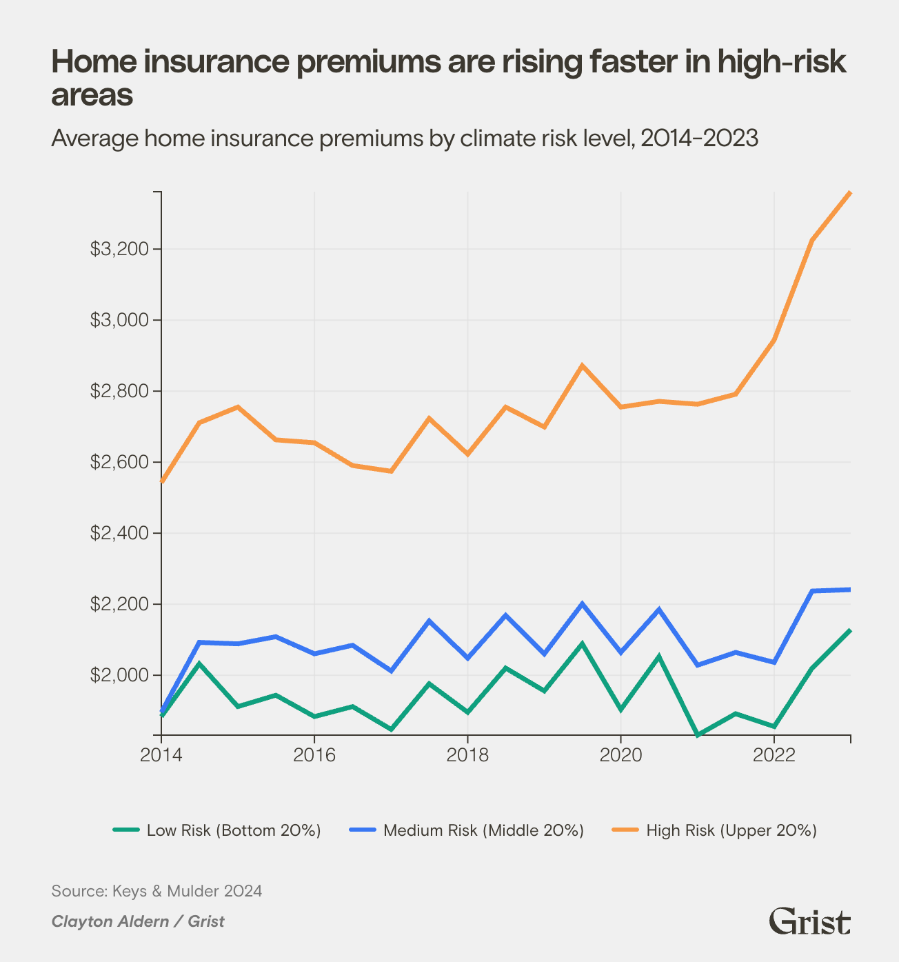
Home insurance premiums are rising faster in high-risk areas
Average home insurance premiums by climate risk level, 2014-2023
(function() {
const INIT_KEY = ‘__grist_insurance_premiums_initialized__’;
if (window[INIT_KEY]) { return; }
window[INIT_KEY] = true;
const COLORS = {
TEXT: ‘var(–color-primary)’,
LINES: {
‘1’: ‘var(–color-turquoise)’,
‘3’: ‘var(–color-cobalt)’,
‘5’: ‘var(–color-orange)’
}
};
const initialSvgHeight = 450;
const svg = d3.select(‘#premiums-chart’);
// Raw data parsed from CSV
const rawData = [
{ date: ‘1/1/14’, premium: 2542.17, quintile: 5 },
{ date: ‘7/1/14’, premium: 2710.84, quintile: 5 },
{ date: ‘1/1/15’, premium: 2755.02, quintile: 5 },
{ date: ‘7/1/15’, premium: 2662.65, quintile: 5 },
{ date: ‘1/1/16’, premium: 2654.62, quintile: 5 },
{ date: ‘7/1/16’, premium: 2590.36, quintile: 5 },
{ date: ‘1/1/17’, premium: 2574.30, quintile: 5 },
{ date: ‘7/1/17’, premium: 2722.89, quintile: 5 },
{ date: ‘1/1/18’, premium: 2622.49, quintile: 5 },
{ date: ‘7/1/18’, premium: 2755.02, quintile: 5 },
{ date: ‘1/1/19’, premium: 2698.80, quintile: 5 },
{ date: ‘7/1/19’, premium: 2871.49, quintile: 5 },
{ date: ‘1/1/20’, premium: 2755.02, quintile: 5 },
{ date: ‘7/1/20’, premium: 2771.08, quintile: 5 },
{ date: ‘1/1/21’, premium: 2763.05, quintile: 5 },
{ date: ‘7/1/21’, premium: 2791.16, quintile: 5 },
{ date: ‘1/1/22’, premium: 2943.78, quintile: 5 },
{ date: ‘7/1/22’, premium: 3224.90, quintile: 5 },
{ date: ‘1/1/23’, premium: 3361.45, quintile: 5 },
{ date: ‘1/1/14’, premium: 1883.53, quintile: 1 },
{ date: ‘7/1/14’, premium: 2032.13, quintile: 1 },
{ date: ‘1/1/15’, premium: 1911.65, quintile: 1 },
{ date: ‘7/1/15’, premium: 1943.78, quintile: 1 },
{ date: ‘1/1/16’, premium: 1883.53, quintile: 1 },
{ date: ‘7/1/16’, premium: 1911.65, quintile: 1 },
{ date: ‘1/1/17’, premium: 1847.39, quintile: 1 },
{ date: ‘7/1/17’, premium: 1975.90, quintile: 1 },
{ date: ‘1/1/18’, premium: 1895.58, quintile: 1 },
{ date: ‘7/1/18’, premium: 2020.08, quintile: 1 },
{ date: ‘1/1/19’, premium: 1955.82, quintile: 1 },
{ date: ‘7/1/19’, premium: 2088.35, quintile: 1 },
{ date: ‘1/1/20’, premium: 1903.61, quintile: 1 },
{ date: ‘7/1/20’, premium: 2052.21, quintile: 1 },
{ date: ‘1/1/21’, premium: 1831.33, quintile: 1 },
{ date: ‘7/1/21’, premium: 1891.57, quintile: 1 },
{ date: ‘1/1/22’, premium: 1855.42, quintile: 1 },
{ date: ‘7/1/22’, premium: 2020.08, quintile: 1 },
{ date: ‘1/1/23’, premium: 2128.51, quintile: 1 },
{ date: ‘1/1/14’, premium: 1895.58, quintile: 3 },
{ date: ‘7/1/14’, premium: 2092.37, quintile: 3 },
{ date: ‘1/1/15’, premium: 2088.35, quintile: 3 },
{ date: ‘7/1/15’, premium: 2108.43, quintile: 3 },
{ date: ‘1/1/16’, premium: 2060.24, quintile: 3 },
{ date: ‘7/1/16’, premium: 2084.34, quintile: 3 },
{ date: ‘1/1/17’, premium: 2012.05, quintile: 3 },
{ date: ‘7/1/17’, premium: 2152.61, quintile: 3 },
{ date: ‘1/1/18’, premium: 2048.19, quintile: 3 },
{ date: ‘7/1/18’, premium: 2168.67, quintile: 3 },
{ date: ‘1/1/19’, premium: 2060.24, quintile: 3 },
{ date: ‘7/1/19’, premium: 2200.80, quintile: 3 },
{ date: ‘1/1/20’, premium: 2064.26, quintile: 3 },
{ date: ‘7/1/20’, premium: 2184.74, quintile: 3 },
{ date: ‘1/1/21’, premium: 2028.11, quintile: 3 },
{ date: ‘7/1/21’, premium: 2064.26, quintile: 3 },
{ date: ‘1/1/22’, premium: 2036.14, quintile: 3 },
{ date: ‘7/1/22’, premium: 2236.95, quintile: 3 },
{ date: ‘1/1/23’, premium: 2240.96, quintile: 3 }
];
// Process data
const parseDate = d3.timeParse(‘%m/%d/%y’);
const data = rawData.map(d => ({
date: parseDate(d.date),
premium: +d.premium,
quintile: +d.quintile
}));
// Group by quintile
const dataByQuintile = d3.group(data, d => d.quintile);
const quintileLabels = {
1: ‘Low Risk (Bottom 20%)’,
3: ‘Medium Risk (Middle 20%)’,
5: ‘High Risk (Upper 20%)’
};
const margin = { top: 20, right: 20, bottom: 36, left: window.innerWidth x(d.date))
.y(d => y(d.premium));
x.domain(d3.extent(data, d => d.date));
y.domain(d3.extent(data, d => d.premium));
svg.attr(‘height’, initialSvgHeight);
// Gridlines
svg.append(‘g’)
.attr(‘class’, ‘axis-grid’)
.attr(‘transform’, `translate(${margin.left},${height + margin.top})`)
.call(d3.axisBottom(x).ticks(d3.timeYear.every(2)).tickSize(-height).tickFormat(”));
svg.append(‘g’)
.attr(‘class’, ‘axis-grid’)
.attr(‘transform’, `translate(${margin.left},${margin.top})`)
.call(d3.axisLeft(y).ticks(5).tickSize(-width).tickFormat(”));
const xAxis = g => g
.attr(‘transform’, `translate(${margin.left},${height + margin.top})`)
.call(d3.axisBottom(x).ticks(d3.timeYear.every(2)).tickFormat(d3.timeFormat(‘%Y’)))
.selectAll(‘text’)
.attr(‘class’, ‘insurance-premiums__axis-label’)
.style(‘fill’, COLORS.TEXT)
.style(‘text-anchor’, ‘middle’);
const yAxis = g => g
.attr(‘transform’, `translate(${margin.left},${margin.top})`)
.call(d3.axisLeft(y).ticks(5).tickFormat(d => `$${d3.format(‘,’)(d)}`))
.selectAll(‘text’)
.attr(‘class’, ‘insurance-premiums__axis-label’)
.style(‘fill’, COLORS.TEXT);
svg.append(‘g’).call(xAxis);
svg.append(‘g’).call(yAxis);
const chart = svg.append(‘g’).attr(‘transform’, `translate(${margin.left},${margin.top})`);
// Draw lines for each quintile
dataByQuintile.forEach((values, quintile) => {
const sortedValues = values.sort((a, b) => a.date – b.date);
chart.append(‘path’)
.datum(sortedValues)
.attr(‘class’, ‘line’)
.attr(‘d’, line)
.style(‘stroke’, COLORS.LINES[quintile])
.style(‘fill’, ‘none’);
});
// Add legend
const legend = d3.select(‘#insurance-legend’);
[1, 3, 5].forEach(quintile => {
const item = legend.append(‘div’).attr(‘class’, ‘insurance-legend-item’);
item.append(‘div’)
.attr(‘class’, ‘insurance-legend-color’)
.style(‘background-color’, COLORS.LINES[quintile]);
item.append(‘span’)
.style(‘color’, COLORS.TEXT)
.text(quintileLabels[quintile]);
});
}
if (document.readyState === ‘loading’) {
document.addEventListener(‘DOMContentLoaded’, renderChart);
} else {
renderChart();
}
window.addEventListener(‘resize’, renderChart);
})();
Insurance premiums for American homes have risen 30 percent on average since 2020. The increase hasn’t been felt equally across the country. Homeowners in areas with the highest risk of natural disasters — along the coasts and in the middle of the country where tornados are common — have seen their premiums rise the most (controlling for all other factors). Households in some parts of Florida, for example, have seen their insurance premiums rise $4,000 or more.
.population-movement {
–color-primary: #3c3830;
–color-secondary: #777;
–color-orange: #F79945;
–color-turquoise: #12A07F;
–color-fuchsia: #AC00E8;
–color-cobalt: #3977F3;
–color-earth: #3c3830;
–typography-primary: “PolySans”, Arial, sans-serif;
–typography-secondary: “Basis Grotesque”, Arial, sans-serif;
–spacing-base: 10px;
box-sizing: border-box;
font-family: var(–typography-secondary);
margin: 3rem auto 1.5rem auto;
padding: 0;
position: relative;
width: 100%;
}
.population-movement * { box-sizing: border-box; }
.population-movement__title {
font-family: var(–typography-primary);
font-size: 24px;
margin: var(–spacing-base) 0;
}
.population-movement__subtitle {
font-family: var(–typography-secondary);
color: var(–color-primary);
font-size: 18px;
margin: 0 0 var(–spacing-base);
}
.population-movement__axis-label {
color: var(–color-primary);
font-size: 14px;
}
.axis-grid line {
stroke: #e0e0e0;
stroke-opacity: 0.7;
shape-rendering: crispEdges;
}
.axis-grid .domain { stroke: none; }
.movement-legend {
font-family: var(–typography-secondary);
font-size: 12px;
display: flex;
justify-content: center;
margin-top: 0px;
margin-bottom: 25px;
gap: 20px;
flex-wrap: wrap;
}
.movement-legend-item {
display: flex;
align-items: center;
gap: 5px;
}
.movement-legend-color {
width: 15px;
height: 15px;
border-radius: 2px;
}
.population-movement__footer { display: flex; justify-content: space-between; align-items: flex-end; margin-top: 8px; }
.population-movement__credits { display: flex; flex-direction: column; }
.population-movement__source { color: var(–color-secondary); font-size: 12px; margin-top: 0; display: inline-block; }
.population-movement__credit { color: var(–color-secondary); font-size: 12px; margin-top: 3px; font-style: italic; font-weight: bold; display: inline-block; }
.population-movement__logo { height: 20px; width: auto; margin-left: auto; padding-right: 20px; margin-right: 0; margin-bottom: 0; }
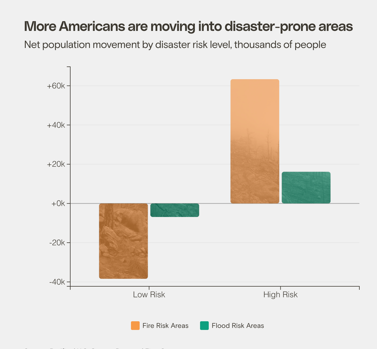
More Americans are moving into disaster-prone areas
Net population movement by disaster risk level, thousands of people
(function() {
const INIT_KEY = ‘__grist_population_movement_initialized__’;
if (window[INIT_KEY]) { return; }
window[INIT_KEY] = true;
const COLORS = {
TEXT: ‘var(–color-primary)’,
FIRE: ‘var(–color-orange)’,
FLOOD: ‘var(–color-turquoise)’,
OPACITY: 0.65
};
const initialSvgHeight = 450;
const svg = d3.select(‘#movement-chart’);
const BAR_RADIUS = 4;
// Data from movement.csv – converted to thousands
const rawData = [
{ risk: ‘Low Risk’, disaster: ‘Fire’, amount: -38.401 },
{ risk: ‘Low Risk’, disaster: ‘Flood’, amount: -6.892 },
{ risk: ‘High Risk’, disaster: ‘Fire’, amount: 63.365 },
{ risk: ‘High Risk’, disaster: ‘Flood’, amount: 16.144 }
];
const data = rawData;
const margin = { top: 20, right: 20, bottom: 50, left: window.innerWidth width) {
line.pop();
tspan.text(line.join(‘ ‘));
line = [word];
tspan = text.append(‘tspan’).attr(‘x’, 0).attr(‘y’, y).attr(‘dy’, ++lineNumber * (lineHeight / 14) + dy + ’em’).text(word);
}
}
});
}
function renderChart() {
svg.selectAll(‘*’).remove();
d3.select(‘#movement-legend’).selectAll(‘*’).remove();
const node = svg.node();
const styleWidth = parseInt(svg.style(‘width’));
const containerWidth = node ? node.getBoundingClientRect().width : (isNaN(styleWidth) ? 600 : styleWidth);
const width = containerWidth – margin.left – margin.right;
const height = initialSvgHeight – margin.top – margin.bottom;
svg.attr(‘height’, initialSvgHeight);
// Create grouped data structure for grouped bar chart
const groups = d3.group(data, d => d.risk);
const risks = Array.from(groups.keys());
const disasters = [‘Fire’, ‘Flood’];
const x0 = d3.scaleBand().domain(risks).range([0, width]).padding(0.2);
const x1 = d3.scaleBand().domain(disasters).range([0, x0.bandwidth()]).padding(0.05);
const yExtent = d3.extent(data, d => d.amount);
const y = d3.scaleLinear()
.domain([Math.min(yExtent[0] * 1.1, 0), Math.max(yExtent[1] * 1.1, 0)])
.range([height, 0]);
// Zero line
svg.append(‘line’)
.attr(‘x1’, margin.left)
.attr(‘x2’, margin.left + width)
.attr(‘y1’, margin.top + y(0))
.attr(‘y2’, margin.top + y(0))
.attr(‘stroke’, ‘#333’)
.attr(‘stroke-width’, 1);
// Gridlines
svg.append(‘g’)
.attr(‘class’, ‘axis-grid’)
.attr(‘transform’, `translate(${margin.left},${margin.top})`)
.call(d3.axisLeft(y).ticks(5).tickSize(-width).tickFormat(”));
const xAxis = g => {
g.attr(‘transform’, `translate(${margin.left},${height + margin.top})`)
.call(d3.axisBottom(x0));
// Wrap tick labels on small widths
const maxWidth = Math.min(80, Math.max(48, width / risks.length – 6));
g.selectAll(‘.tick text’)
.attr(‘class’, ‘population-movement__axis-label’)
.style(‘fill’, COLORS.TEXT)
.style(‘text-anchor’, ‘middle’)
.call(wrapSvgText, maxWidth, 14);
};
const yAxis = g => g
.attr(‘transform’, `translate(${margin.left},${margin.top})`)
.call(d3.axisLeft(y).ticks(5).tickFormat(d => d >= 0 ? `+${d}k` : `${d}k`))
.selectAll(‘text’)
.attr(‘class’, ‘population-movement__axis-label’)
.style(‘fill’, COLORS.TEXT);
svg.append(‘g’).call(xAxis);
svg.append(‘g’).call(yAxis);
const chartGroup = svg.append(‘g’).attr(‘transform’, `translate(${margin.left},${margin.top})`);
// Image fills using masks
const defs = chartGroup.append(‘defs’);
const grayFilter = defs.append(‘filter’).attr(‘id’, ‘movementGreyscale’);
grayFilter.append(‘feColorMatrix’).attr(‘type’, ‘saturate’).attr(‘values’, ‘0’);
const barsMask = defs.append(‘mask’).attr(‘id’, ‘movementBarsMask’);
data.forEach((d, i) => {
const xPos = x0(d.risk) + x1(d.disaster);
const yPos = d.amount >= 0 ? y(d.amount) : y(0);
const barHeight = Math.abs(y(d.amount) – y(0));
barsMask.append(‘rect’)
.attr(‘x’, xPos)
.attr(‘y’, yPos)
.attr(‘width’, x1.bandwidth())
.attr(‘height’, barHeight)
.attr(‘rx’, BAR_RADIUS)
.attr(‘ry’, BAR_RADIUS)
.attr(‘fill’, ‘white’);
});
chartGroup.append(‘image’)
.attr(‘xlink:href’, ‘https://grist.org/wp-content/uploads/2025/08/intricate-explorer-XgorRqQg6PI-unsplash.jpg’)
.attr(‘x’, 0)
.attr(‘y’, 0)
.attr(‘width’, width)
.attr(‘height’, height)
.attr(‘preserveAspectRatio’, ‘xMidYMid slice’)
.attr(‘mask’, ‘url(#movementBarsMask)’)
.attr(‘filter’, ‘url(#movementGreyscale)’);
// Draw bars
chartGroup.selectAll(‘.bar’)
.data(data)
.enter().append(‘rect’)
.attr(‘class’, ‘bar’)
.attr(‘x’, d => x0(d.risk) + x1(d.disaster))
.attr(‘y’, d => d.amount >= 0 ? y(d.amount) : y(0))
.attr(‘width’, x1.bandwidth())
.attr(‘height’, d => Math.abs(y(d.amount) – y(0)))
.attr(‘rx’, BAR_RADIUS)
.attr(‘ry’, BAR_RADIUS)
.style(‘fill’, d => d.disaster === ‘Fire’ ? COLORS.FIRE : COLORS.FLOOD)
.style(‘opacity’, COLORS.OPACITY);
// Add legend
const legend = d3.select(‘#movement-legend’);
const fireItem = legend.append(‘div’).attr(‘class’, ‘movement-legend-item’);
fireItem.append(‘div’)
.attr(‘class’, ‘movement-legend-color’)
.style(‘background-color’, COLORS.FIRE);
fireItem.append(‘span’)
.style(‘color’, COLORS.TEXT)
.text(‘Fire Risk Areas’);
const floodItem = legend.append(‘div’).attr(‘class’, ‘movement-legend-item’);
floodItem.append(‘div’)
.attr(‘class’, ‘movement-legend-color’)
.style(‘background-color’, COLORS.FLOOD);
floodItem.append(‘span’)
.style(‘color’, COLORS.TEXT)
.text(‘Flood Risk Areas’);
}
if (document.readyState === ‘loading’) {
document.addEventListener(‘DOMContentLoaded’, renderChart);
} else {
renderChart();
}
window.addEventListener(‘resize’, renderChart);
})();
Expensive disasters are striking more frequently, but Americans are also increasingly putting themselves in harm’s way. In 2023, roughly 63,000 people moved into counties at high risk for wildfires and about 16,000 moved into flood-prone counties, many of them in search of lower taxes and more ample and affordable housing. The opposite trend unfolded in low-risk areas: Some 38,000 people left the country’s low-fire-risk counties and nearly 7,000 people left low-flood-risk counties.
-
Illegal price-gouging is rampant after disasters. Can it be stopped?
-
Two years after a wildfire took everything, Maui homeowners are facing a new threat: Foreclosure

const css = `
:root {
–rs-color-primary: #3c3830;
–rs-color-secondary: #dfdfdf;
–rs-typography-primary: “PolySans”, sans-serif;
–rs-typography-secondary: “GT Super Text”, serif;
}
.rs-callout {
position: relative;
max-width: 600px;
margin: 2rem auto;
}
@media (min-width: 1440px) {
.rs-callout {
position: absolute;
max-width: 300px;
left: 0;
}
}
.rs-callout__title {
color: var(–rs-color-primary);
font-family: var(–rs-typography-primary);
font-weight: 600;
margin-bottom: 0.375rem;
font-size: 1.25rem; /* 20px */
line-height: 1.75rem; /* 28px */
}
.rs-callout__features {
list-style: none;
padding: 0;
border-top: 1px solid var(–rs-color-primary);
border-bottom: 1px solid var(–rs-color-primary);
margin: 0;
}
.rs-callout__features > .rs-callout__feature + .rs-callout__feature {
border-top: 1px solid var(–rs-color-secondary);
}
.rs-callout__feature {
padding: 1.5rem 0;
/* Grist Global CSS override. */
padding-left: 0 !important;
margin-top: 0 !important;
}
.rs-callout__feature::before {
/* Grist Global CSS override. */
content: “” !important;
}
.rs-callout__feature .rs-callout__feature-link {
display: flex;
justify-content: space-between;
gap: 2rem;
text-decoration: none;
/* Grist Global CSS override. */
border: none;
}
.rs-callout__feature .rs-callout__feature-link:hover {
/* Grist Global CSS override. */
border: none;
}
@media (min-width: 1440px) {
.rs-callout__feature-link {
gap: 1rem;
}
}
.rs-callout__feature-title {
color: var(–rs-color-primary);
font-family: var(–rs-typography-secondary);
margin: 0;
font-size: 0.875rem; /* 14px */
line-height: 1.25rem; /* 20px */
}
@media (min-width: 612px) {
.rs-callout__feature-title {
font-size: 1.125rem; /* 18px */
line-height: 1.75rem; /* 28px */
}
}
@media (min-width: 1024px) {
.rs-callout__feature-title {
font-size: 1.125rem; /* 18px */
line-height: 1.75rem; /* 28px */
}
}
@media (min-width: 1440px) {
.rs-callout__feature-title {
font-size: 0.875rem; /* 14px */
line-height: 1.25rem; /* 20px */
}
}
.rs-callout__feature-img {
width: 10rem;
height: auto;
aspect-ratio: 16 / 9;
object-fit: cover;
}
@media (min-width: 612px) {
.rs-callout__feature-img {
width: 12rem;
}
}
@media (min-width: 768px) {
.rs-callout__feature-img {
width: 14rem;
}
}
@media (min-width: 1440px) {
.rs-callout__feature-img {
width: 8rem;
}
}
.rs-callout__title-logo {
max-width: 80%; /* default size for regular screens */
height: auto;
}
@media (max-width: 768px) {
.rs-callout__title-logo {
max-width: 45%; /* smaller on small screens */
}
}
@media (min-width: 1440px) {
.rs-callout__title-logo {
max-width: 80%; /* slightly smaller on very large screens */
}
}
`;
const style = document.createElement(“style”);
style.appendChild(document.createTextNode(css));
document.head.appendChild(style);

There is a way to break the cycle. By the federal government’s own calculations, every dollar spent on preparing for a disaster before it hits saves $6 down the line. But the Trump administration has turned that sound logic on its head, eliminating the nation’s main streams of disaster preparedness funding and severely weakening FEMA’s ability to both help states prepare for disasters and respond to them once they’ve struck.
Since April, the Trump administration has cut $750 million in new resilience funding and clawed back nearly $900 million in grant funding already promised but not yet disbursed to states for improvements like upgrading stormwater systems, conducting prescribed burns, and building flood-control systems. About 10 percent of FEMA’s staff has been laid off, fired, or put on leave, and the agency could lose up to 30 percent of its workforce by the end of the year.
Millions of people, particularly those in the most climate-vulnerable parts of the country, stand to lose as a result of the confluence of climate-driven extreme weather events and the Trump administration’s disaster-resilience reforms. But other parties stand to gain.
“There’s many reasons we don’t have global peace, and part of it is that war is profitable,” said Victoria Salinas, who led FEMA’s resilience initiatives under former president Joe Biden. “Similarly, disaster response is profitable. For some.”
.tf-v1-widget iframe{
padding-bottom: 90px;
}
toolTips(‘.classtoolTips3′,’Carbon dioxide, methane, nitrous oxide, and other gases that prevent heat from escaping Earth’s atmosphere. Together, they act as a blanket to keep the planet at a liveable temperature in what is known as the “greenhouse effect.” Too many of these gases, however, can cause excessive warming, disrupting fragile climates and ecosystems.’); toolTips(‘.classtoolTips10′,’A scarce blue metal that helps battery cathodes store large amounts of energy without overheating or collapsing. It is a key component of lithium-ion batteries. ‘);
This story was originally published by Grist with the headline A look at the growing ‘disaster economy’ turning crisis into cash on Aug 12, 2025.