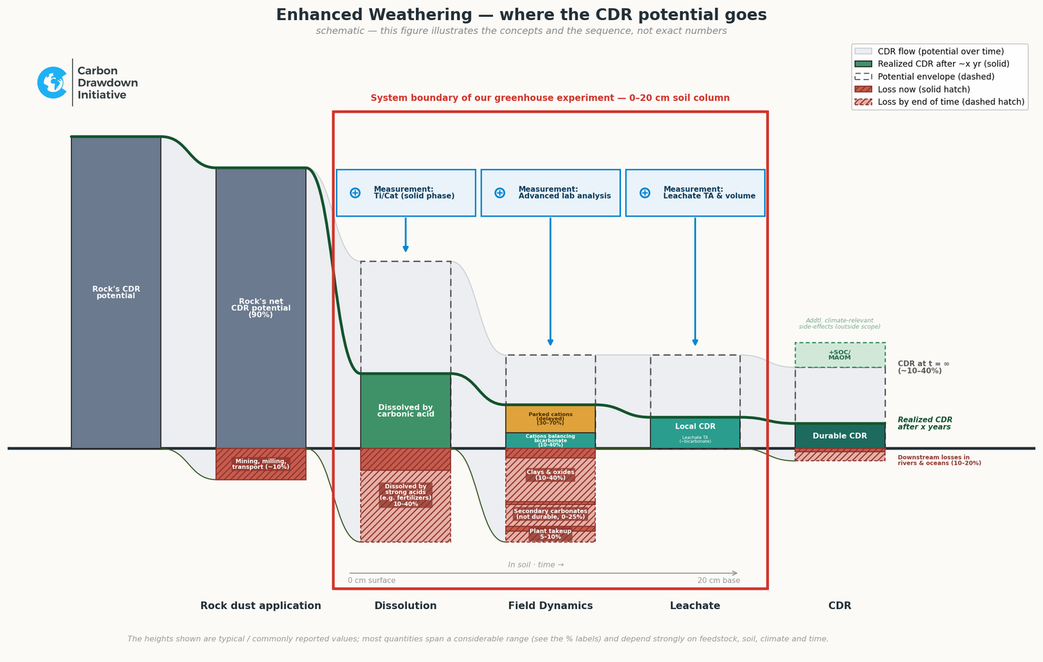
When you spread finely ground silicate rock dust on a field, the material carries a theoretical capacity to pull CO₂ out of the air. As the rock weathers it releases base cations, those cations hold dissolved CO₂ in the form of bicarbonate, and that bicarbonate can eventually be stored away for a very long time. The interesting — and genuinely hard — question is how much of that theoretical capacity actually survives all the way to durable carbon removal. The diagram above follows one batch of rock dust from left to right and shows where the potential is spent along the way.
This is a concept map, not a scoreboard. The height of each block is illustrative. Most of these quantities vary enormously from one soil to the next, from season to season and from year to year, and several of them are difficult to measure at all. So the picture is meant to be read for the relationships and the sequence of events, not for the precise size of any single block. Where a block carries a percentage it is a wide “typical” range; the figures that can be pinned to the literature are taken from the recent 74-author systematic review of enhanced weathering by Suhrhoff and colleagues (2026), the current best synthesis of the field.
A quick walk along the flow. Making and moving the rock dust already costs some CO₂. Across the life-cycle studies the review compiles, these emissions “range from 1.1 to 215 kg CO2-eq t rock⁻¹ (mean = 51.6, median = 33.15),” with “grinding and transport … averaging 41% and 39.4% of total EW life cycle GHG emissions” — on the order of ten percent of a typical rock’s removal potential, and large enough that they “can even eliminate net removals altogether.”
In the soil the rock slowly dissolves, and what dissolves splits in the soil water: some cations immediately balance dissolved bicarbonate — the productive, CO₂-carrying form — while a larger share is temporarily parked on the soil’s exchange sites (delayed, but not lost: it can be released again later). What finally leaves the bottom of the root zone as dissolved alkalinity is what can be measured in the drainage water; further downstream a slice is lost again in rivers and the ocean, for which the review concludes that “an average value of ~15-20% cumulative loss (both rivers and ocean) is more appropriate for long-term storage.” A separate bonus — extra carbon stored in the soil itself — can sit on top, but it lies outside the boundary drawn here.
The most important message is below the line. Three permanent loss channels decide almost everything. The first is dissolution driven by strong acids — the nitric and sulfuric acid that arrive with fertiliser and acid deposition — because “protons derived from strong acids can drive mineral dissolution without consuming atmospheric CO2, thereby reducing net CDR efficiency,” and in croplands “nitric acid generated during fertiliser nitrification represents a major source of strong acidity.” The second is the secondary minerals, since “the formation of secondary minerals—especially clays—hinders the efficiency of EW, such that less CDR is realised per unit of feedstock applied.” The third is secondary carbonates, and it deserves a word because it is tempting to count it as storage: chalk-like carbonate can form in the soil and does contain carbon, but it is not durable. In the review’s words, “the precipitation of solid carbonate minerals reduces the efficiency of EW by nearly half due to the re-release of CO2,” making it “a transient rather than permanent atmospheric CO2 sink”; at catchment scale “carbonate precipitation could reduce the CDR potential of EW by 16–27%.” Accordingly, in modern carbon accounting “secondary carbonate formation is mostly presented as a potential loss of CDR potential” — which is why it sits on the loss side of the diagram, next to the clays and oxides.
Whatever ends up in these three channels is gone for the purpose of removal. The ranges on the figure — very roughly 10–40 % for strong acids, 10–40 % for clays and oxides, and up to about a quarter for secondary carbonates — are our own field-typical estimates informed by the review rather than single quoted values, and they are wide because these losses swing from almost nothing in a favourable soil to almost everything in an unfavourable one; in the worst case they can consume nearly the entire benefit. These, therefore, are the first numbers worth measuring well: if they are large, nothing else on the diagram can rescue the result.
Tellingly, the review flags exactly these as the weakest links: “Significant uncertainty remains regarding the magnitude, persistence, and timing of loss processes after initial CDR has occurred, including secondary phase formation and cation exchange.” The biggest levers on the outcome are also the ones we currently know least about — the core message of the picture.
Only once those are pinned down does the rest become interesting: how much of the rock actually dissolves through the productive pathway (weak carbonic acid, formed from CO₂ and water), and how much of that is merely delayed. The delay can be long — “in large parts of the U.S. Corn Belt and Great Plains, less than 50% of CDR potential is realised within the first decade after EW deployment” — but delayed is not the same as lost.
So how much of a rock’s theoretical capacity survives all the way to durable removal at t = ∞? There is no single measured figure: the review reports removal as an annual flux, where “area-normalized CDR fluxes have a median value of 0.84 tonnes of carbon dioxide per hectare per year,” rather than as a fraction of the theoretical maximum. Working the losses through the chain gives a plausible long-run figure of very roughly 10–40 % of the rock’s chemical potential — a derived number, not a measured one, often nearer the lower end, and close to zero where the losses are large.
That, in the end, is what the figure is for: a map of where to point the instruments — and it marks three measurement windows. Early on, a solid-phase mass balance (the Ti/Ca-type method) tracks how much feedstock has weathered. It is worth being precise about what it sees: it captures the total dissolution, including the fraction driven by strong acids, so on its own it over-states the removal — the strong-acid share has to be subtracted separately. In the middle, telling apart the field pools — what is parked, what is locked into clays and oxides, what has precipitated as carbonate — calls for advanced soil analysis, a demanding suite of techniques that is still partly in development. And at the outflow, the durable signal is the leachate alkalinity together with the drainage volume. That volume is deceptively hard to measure directly in an open field, though it can be derived from hydrogeological models that have been developed and refined over decades; in our greenhouse and lysimeter setups, by contrast, we can measure it directly and very precisely — which is exactly why controlled experiments remain so valuable for closing the balance. Between these windows sit the losses that can quietly erase the whole exercise. Get those right first, and everything to the right of them is refinement.
The figure is schematic: it illustrates the concepts and the sequence, not exact numbers. Block heights are typical values with wide ranges that depend strongly on feedstock, soil, climate and time. Quoted figures are verbatim from Suhrhoff et al. (2026); the 10–40 % end-of-time estimate and the individual loss ranges are our own, derived from that review.
Reference: T. J. Suhrhoff, C. Dietzen, T. Kukla, et al. (2026), An Ecosystem of Carbon Dioxide Removal Reviews – Part 3: Enhanced Weathering, CDRXIV preprint #417 — cdrxiv.org/preprint/417.